We post-trained populations of models to develop complementary capabilities. This extends scaling beyond a single model: we can train more models, not just bigger ones.
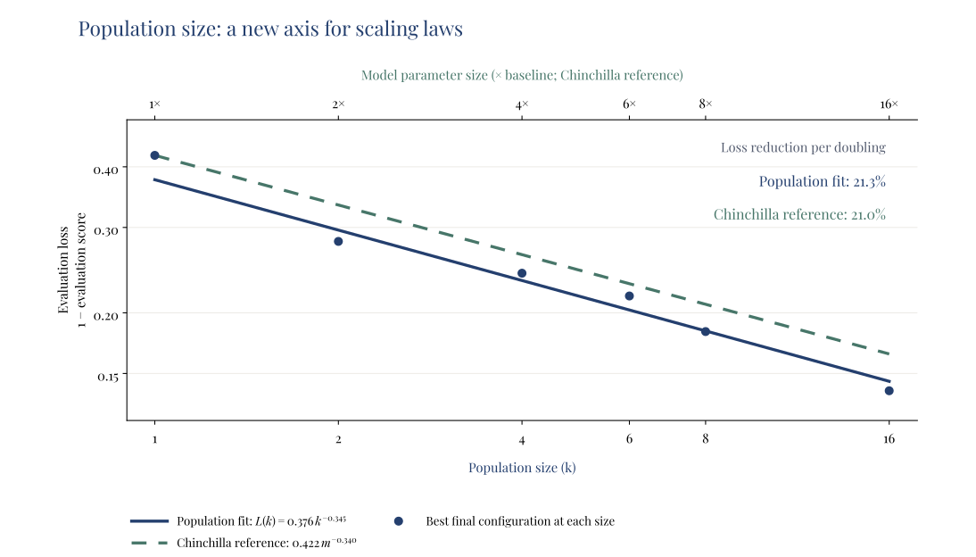
2× the number of models trained ≈ 2.02× the parameters in one model, measured by proportional loss reduction.
TLDR
- We fitted a new scaling law with the number of models trained on the x-axis. Its exponent came out remarkably close to Chinchilla’s: 0.345 vs. 0.34. The comparison is between our evaluation loss and Chinchilla’s reducible language-model loss; the Chinchilla scaling also requires 2.35× the training data.
- At eight models, the diversified population scores 81.70%, versus 71.04% for eight individually trained models and 72.65% for one trained reference model sampled eight times.
- At sixteen models, 22 evaluation tasks have an exact answer from only one member, showing how individual specializations contribute to the population.
The evaluation score averages the best response available per task across three equally weighted benchmarks, using the known answers for scoring. Evaluation loss is one minus that score expressed as a fraction; exact-match coverage is the percentage of tasks with at least one exact answer.
This is the first post in Banbury Road's series on training a civilization of diversified models: end-to-end parameter learning that develops specialization without assigning predefined specialist roles.
What another model contributes
Suppose two models each answer 60 of 100 questions correctly. If they succeed on exactly the same questions, their combined coverage is still 60. If they share only 40 correct answers, their combined coverage is 80. The individual accuracies are identical. The overlap between their successes changes the value of the population.
This makes complementarity a training objective worth pursuing. A model contributes when it produces a useful answer that other members miss. The population's score depends on both the capabilities of its members and how those capabilities are distributed.
Our approach makes the population part of the training process. Members share a pretrained source, and their parameters learn from task outcomes. We use emergent specialization to describe the task-dependent differences that develop through this training without prescribed specialist roles.
Scaling population capability
Familiar pretraining scaling laws describe how loss falls as we increase model parameters, training data, or compute. Chinchilla's fitted law describes the joint effects of model size and training data. We investigate population size as an additional axis: train more models to develop complementary capabilities while keeping each model's parameter count fixed.
Final scores rise across the tested population sizes, including when the training configuration is held fixed. The best observed configuration at each size gives:
| Population size | Final evaluation score | Evaluation loss |
|---|---|---|
| 1 | 57.76% | 0.4224 |
| 2 | 71.92% | 0.2808 |
| 4 | 75.86% | 0.2414 |
| 6 | 78.33% | 0.2167 |
| 8 | 81.70% | 0.1830 |
| 16 | 86.18% | 0.1382 |
Every point is a final outcome of the complete training procedure, including the training that establishes initial diversity.
Loss makes progress near perfect performance visible. Improving exact correctness from 90% to 95% halves the loss; improving from 60% to 70% reduces it by a quarter. Relative loss reduction captures this difference, which absolute score gains obscure.
Let be population size and the final evaluation score. We fit all five sizes—2, 4, 6, 8, and 16—jointly, using the best observed configuration at each size. Least-squares regression in log space gives:
Each doubling reduces evaluation loss by 21.3% in the fitted trend. The exponent's 95% interval is 0.265–0.462, with a log-space of 0.965. These estimates describe the observed population range at its full response budget: one answer per member.
The trend also holds with a training configuration fixed across sizes 4, 6, 8, and 16: that fit gives an exponent of 0.333, or 20.6% lower loss per doubling. Including size one in the best-configuration fit gives an exponent of 0.379, or 23.1% lower loss per doubling. The result is supported by multiple population sizes and both ways of selecting the training configuration.
The parameter multiplier in the opening comparison follows from the two fitted exponents:
This matches proportional reductions in our evaluation loss and Chinchilla's reducible language-model loss; it does not equate their benchmark performance.
At the measured endpoints, eight to sixteen models reduces evaluation loss by 24.49%. Tasks with no exact answer fall from 60 to 47, a 21.67% reduction. This comparison uses eight and sixteen answers respectively. At a fixed budget of eight answers, a uniform subset of the sixteen-model population scores 81.04%, close to the eight-model population's 81.70%.
Better combined performance from weaker average members
We compared two fully trained populations of eight models. The reference models were trained individually, retaining the shared pretrained source and overall experimental setup, but without the population interaction used by our method.
| Eight-model training condition | Mean individual evaluation score | Population evaluation score |
|---|---|---|
| Trained individually | 55.31% | 71.04% |
| Diversified | 47.71% | 81.70% |
The diversified population gained 10.66 percentage points even though its average member scored lower. The paired 95% interval for the population gain is 7.29–14.29 points.
Both conditions used population size eight. Evaluating only the average member would have ranked the training conditions in the opposite order. Evaluating the population reveals the value of their combined answers.
At population size eight, the diversified population also outperforms one trained reference model sampled eight times:
| Method | Population size | Evaluation score | Exact-match coverage |
|---|---|---|---|
| One trained reference model, sampled eight times | 1 | 72.65% | 69.53% |
| Diversified population | 8 | 81.70% | 79.17% |
The population gains 9.05 percentage points in evaluation score and leaves 31.6% fewer tasks without an exact answer. Reference scores average best-of-eight results calculated separately for each of the eight trained reference models; each result uses eight responses from that one model.
The largest gains are in classification coverage. At population size eight, TweetEval rises from 77.21% to 95.83% and SuperGPQA from 59.77% to 67.71%, compared with eight samples from one trained model. MuSiQue changes much less, from 80.97% to 81.56%.
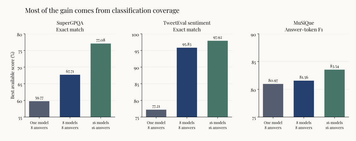
This identifies where the population adds the most value in the current evaluation: it supplies correct classification answers that repeated sampling from an individual model misses.
How specialization appears across the population
The sixteen-model population supplies direct evidence of complementary answers: 22 tasks have an exact answer from only one member. On 29 tasks, one member supplies the unique highest-scoring response.
The distribution changes during training. We identify the tasks on which each model attains the population's highest positive score. Mean pairwise overlap between these task sets falls from 0.675 at an earlier trained checkpoint to 0.494 at the final checkpoint. Members increasingly supply the best available answer on different subsets of tasks.
We also measure what each member adds to the population. The left panel below averages a model's marginal score contribution over every possible order of adding members—the Shapley allocation. The right panel measures the score lost when that member is removed from the full population.
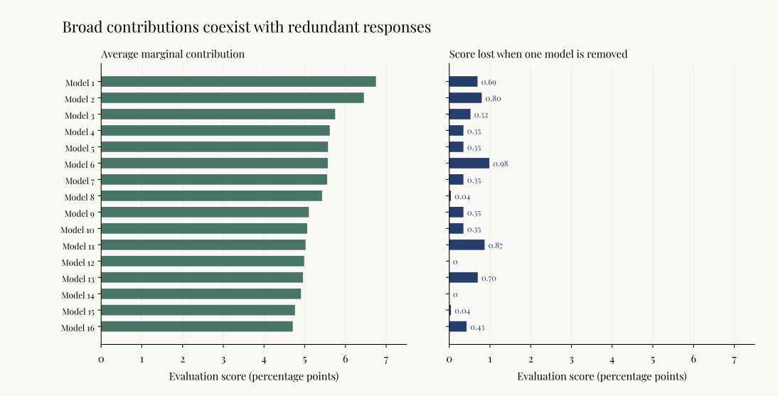
A member can be useful in many smaller subsets even when another member duplicates its answers in the full population. These two measurements distinguish that contribution from the requirement that a particular model be indispensable.
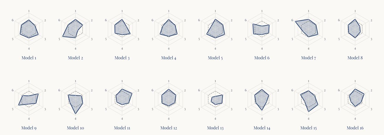
The opening hexagons (Figure 1) show each member's relative task-performance change profile at the final evaluation. Read left to right across the two rows, they follow the same model numbering as Figure 4. All sixteen use the same six fitted coordinates, running clockwise from the top vertex, and signed scale in arbitrary units: center −3.80, dashed hexagon 0 (the population mean), and outer vertices +3.80. Component signs are arbitrary; polygon area is not a capability score. The six-component solution is unstable under resampling, so these are descriptive coordinates rather than established skills.
A separate two-component summary shows greater separation between the middle and final evaluations in all twelve training configurations. Pooled separation increases by 33.4%.
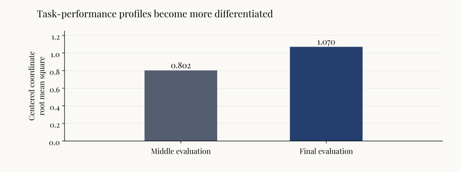
The behavioral result is clear: the members differ in which tasks they answer best, and those differences provide useful coverage for the population. This is the form of specialization measured in this study.
Memory and inference
The population shares a common backbone. A serving implementation can store those shared weights once and retain each member's parameter updates alongside them. Multi-adapter serving systems demonstrate this storage design. S-LoRA
For backbone storage and additional storage per member, total weight storage is . Using our configuration's parameter counts and 16-bit weight storage gives:
| Weight-storage comparison | Analytical result |
|---|---|
| Increase a shared population from eight to sixteen members | 0.6% more |
| Store sixteen shared members instead of sixteen separate full models | 93.7% less |
Doubling the population adds 0.6% to its model-weight storage in this shared design. Serving memory also includes request-specific caches, activations, and temporary buffers, whose sizes depend on the inference workload.
Every selected member performs a model computation. At comparable sequence lengths, sixteen responses require approximately twice the model passes of eight responses. Sharing weights reduces their storage requirement; selecting which members to run determines how many computations are needed.
From available capability to reliable use
Training a population for complementary behavior improves its combined answers, outperforms individually trained populations and repeated sampling from one trained model, and produces a scaling relationship across population sizes. Useful contributions are distributed across the members—even when the average individual score falls.
The next question is how to recover that available performance when the correct answer is unknown. In our next post, we’ll share Banbury Road’s next step toward reliable answer selection. Follow our technical blog series for the next installment.
Evaluation details
All results use a shared training cohort and 288 held-out tasks disjoint from training: 96 each from SuperGPQA, TweetEval sentiment, and MuSiQue-Answerable. Each member supplies one response per task. We score correctness on SuperGPQA and TweetEval, and answer-token F1 on MuSiQue. The eight-answer comparisons hold response count fixed; population scaling increases both training and response budgets.
The scaling fit uses the best observed configuration at each size, selected using this evaluation panel. Configuration selection is repeated when calculating the fit’s confidence interval. The estimates describe the tested population range.
Reported 95% intervals resample tasks or connected task groups. They describe variation across evaluation tasks within this cohort, rather than variation across independent training runs. The eight-model population's 9.05-point advantage over repeated sampling has a paired interval of 6.09–12.26 points.